Embedding
Shows how to create an embedding: choosing what to build, selecting cells and features, setting normalization, standardization and integration, regressing unwanted genes, and choosing a visualization method.
1Open the Embedding tab
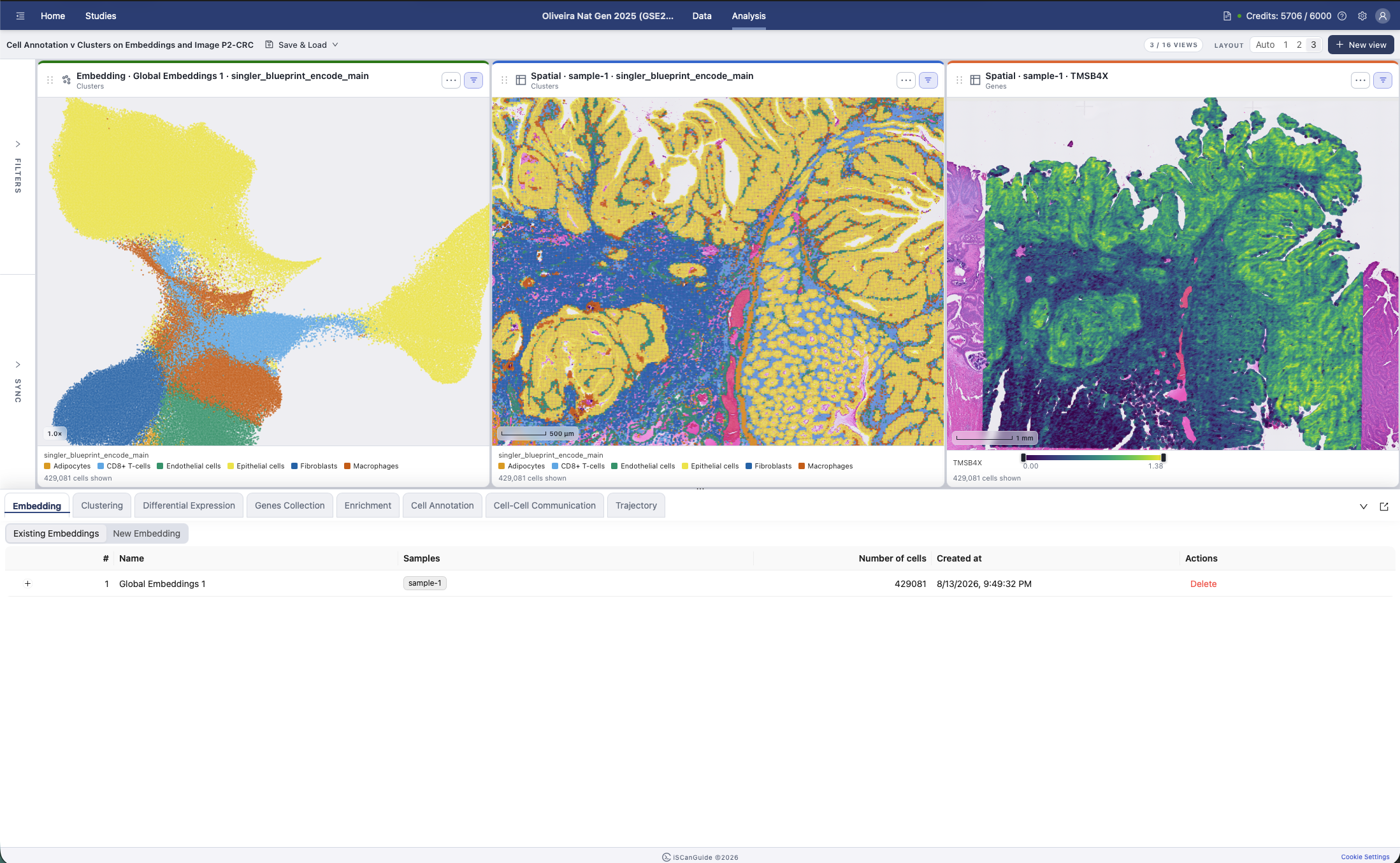
Open Embedding in the bottom drawer. An embedding reduces your data to a small number of dimensions. Clustering and most views are built on one.
2Choose what to build
Custom builds one embedding from the cells you select. The other options build several at once: one per sample, per cluster, per metadata value, or per annotation value.
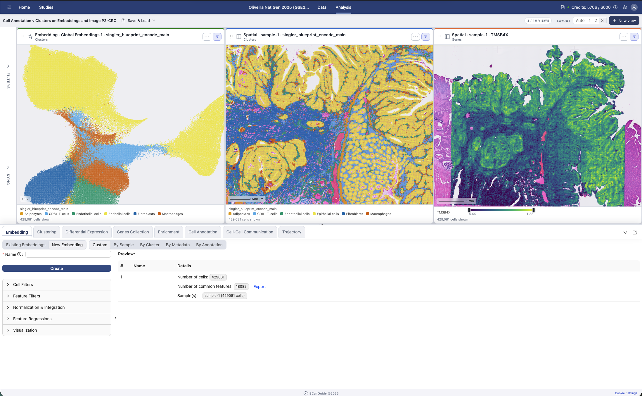
Note: choosing anything other than Custom adds a line confirming what will be created, for example "One embedding will be created for each sample".
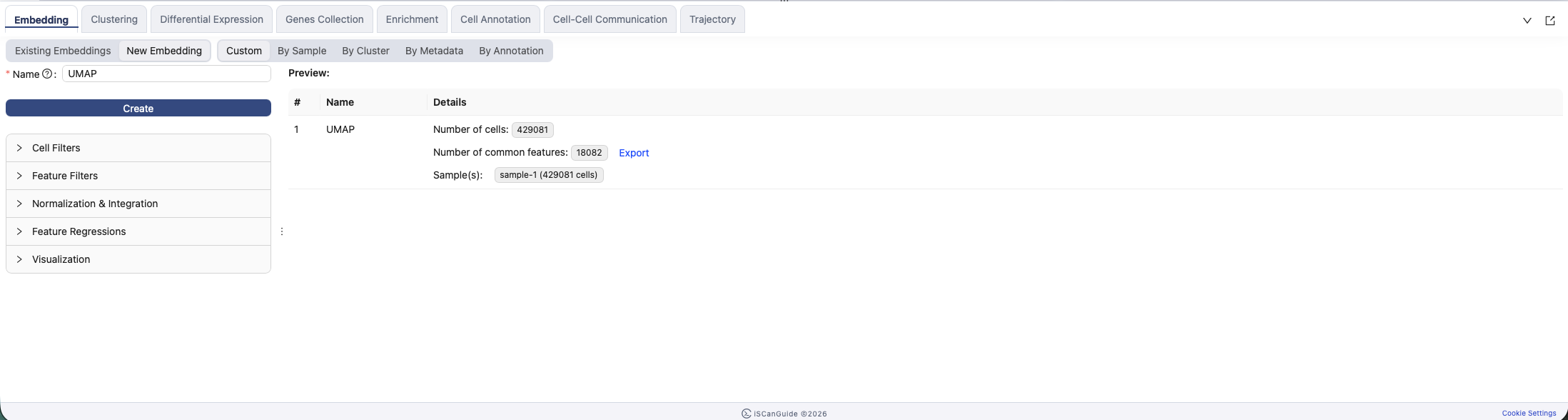
3Name the embedding
Type a name for the embedding. If you are creating several at once, put {sample}, {cluster}, {metadata} or {annotation} into the name and each embedding gets its own value in place of it. The help icon beside Name lists the ones you can use.
4Filter cells
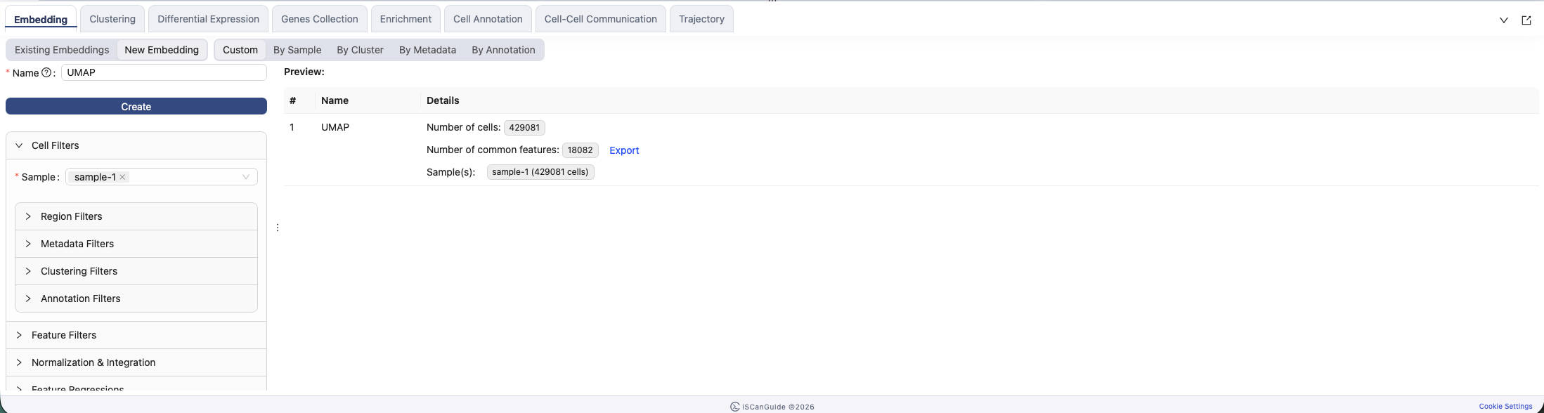
Build the embedding from a subset of cells. Filter by metadata, cluster or annotation, or draw a region on a view and use the cells inside it.
5Filter features
Restrict the embedding to the genes in a gene set. Turn on Filter features by gene set, then pick a collection and the sets within it.
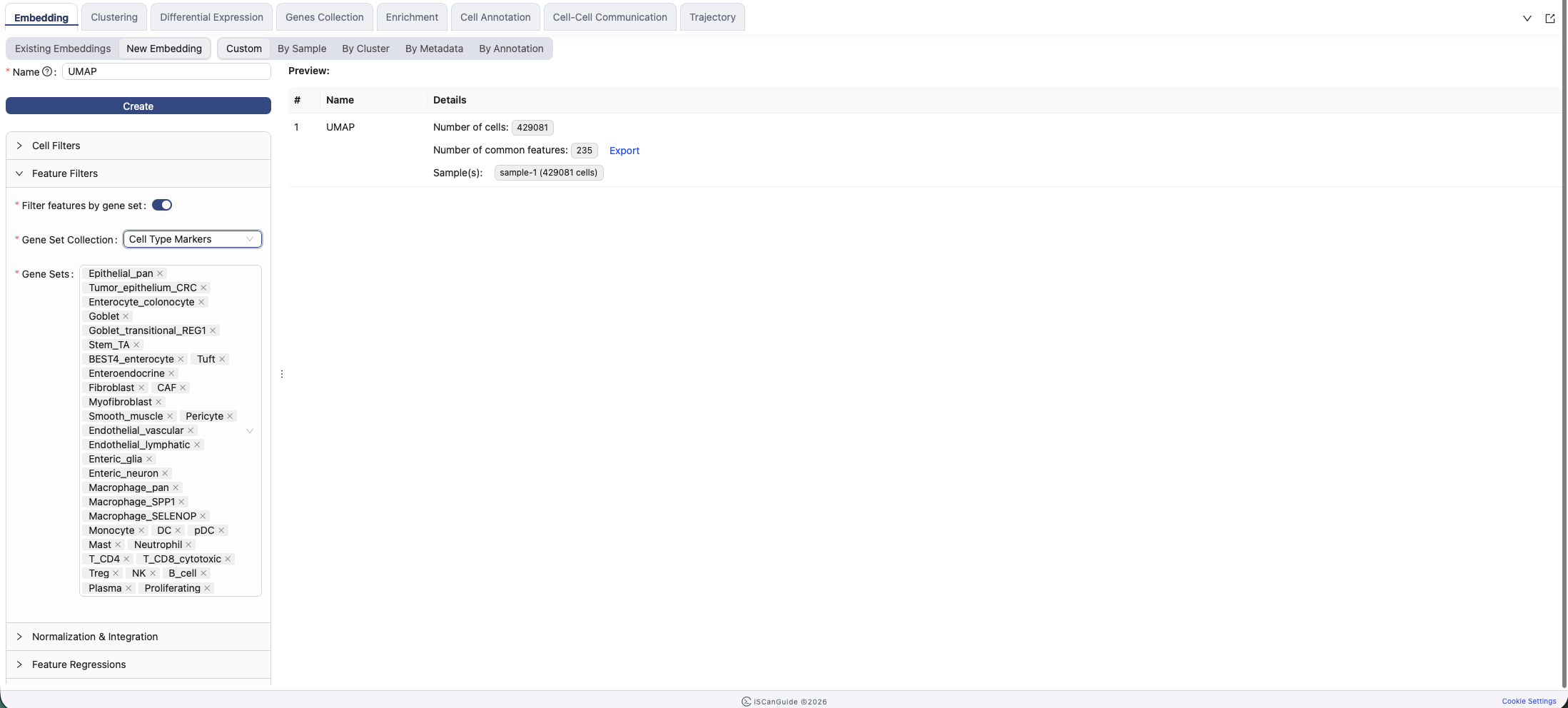
Note: requires at least one gene set collection. See the Genes Collection guide.
6Normalization and standardization
Scaling Factor normalizes each cell for library size across all genes. Feature Standardization then rescales the variable features just before PCA. Standardized centres and unit-variance-scales each gene. Sparse skips the variance scaling, which uses less memory on large datasets.
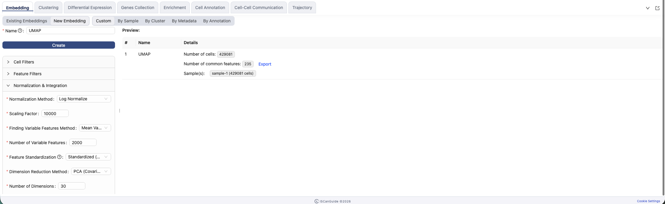
Fields
| Field | Options / range |
|---|---|
Normalization Method | Log Normalize |
Scaling Factor | 1,000 to 1,000,000 |
Finding Variable Features Method | Mean Variance Plot, Highest Dispersion |
Number of Variable Features | 100 to 10,000 |
Feature Standardization | Standardized (center + unit variance), Sparse (centering only, no variance scaling) |
Dimension Reduction Method | PCA tSVD, PCA (Covariance Eigendecomposition), PCA (Arpack) |
Number of Dimensions | 10 to 50 |
PCA tSVD is unavailable when standardization is Sparse: its solver needs dense input.
7Integration
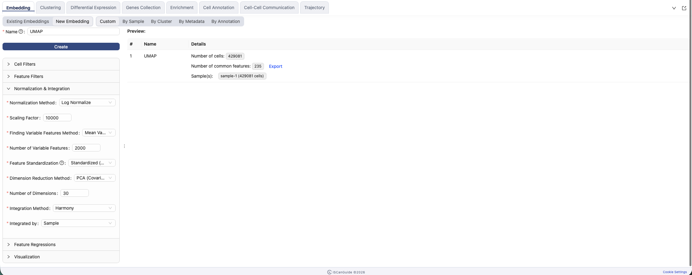
If your data spans several batches, Harmony corrects for them. Choose whether the batches are defined by sample or by a metadata field. Select None for a single dataset.
8Regress unwanted genes
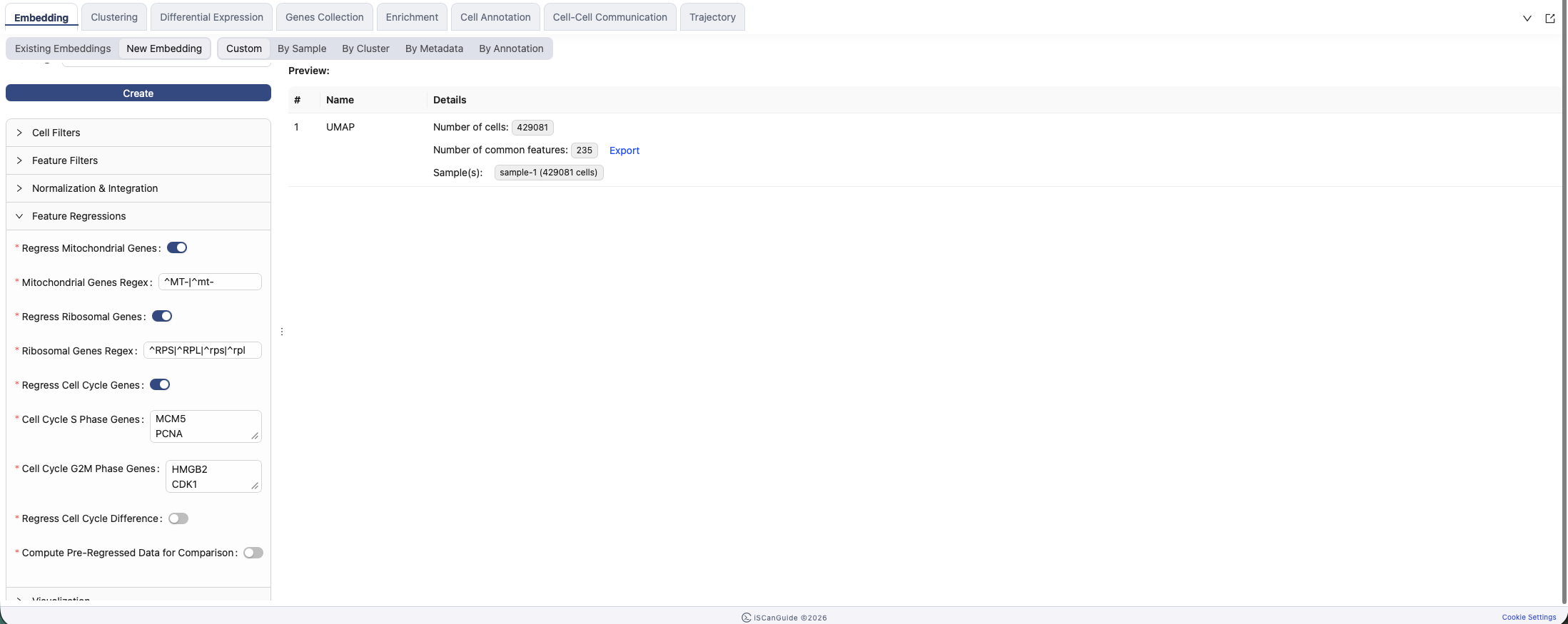
Remove the influence of mitochondrial, ribosomal or cell cycle genes. Each has a default pattern or gene list you can edit. Turn on Compute Pre-Regressed Data for Comparison if you want to see the effect afterwards.
9Choose a visualization method
UMAP is the recommended default and shows both local clusters and the relationships between them. t-SNE separates clusters more sharply but the distances between them are not meaningful. PCA is useful for spotting batch effects.
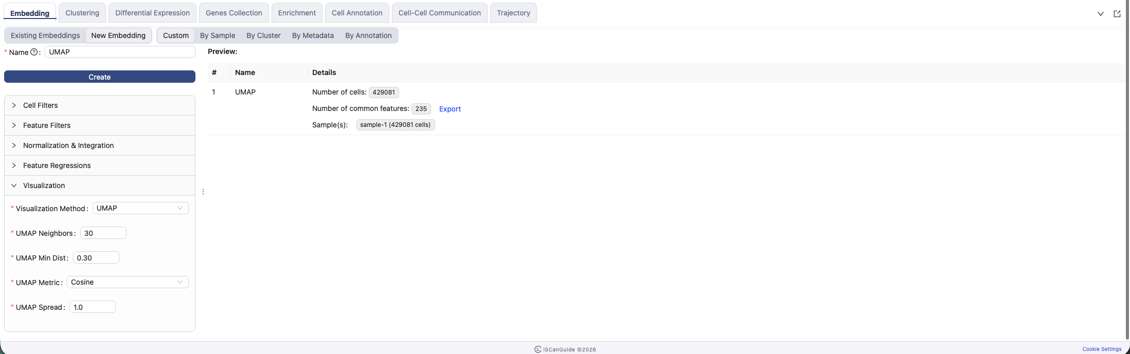
UMAP and t-SNE parameters
| Field | Range |
|---|---|
UMAP Neighbors | 5 to 100, step 5 |
UMAP Min Dist | 0.01 to 0.99, step 0.01 |
UMAP Metric | Cosine, Euclidean |
UMAP Spread | 0.1 to 10, step 0.1 |
t-SNE Perplexity | 5 to 100, step 5 |
10Preview before you create
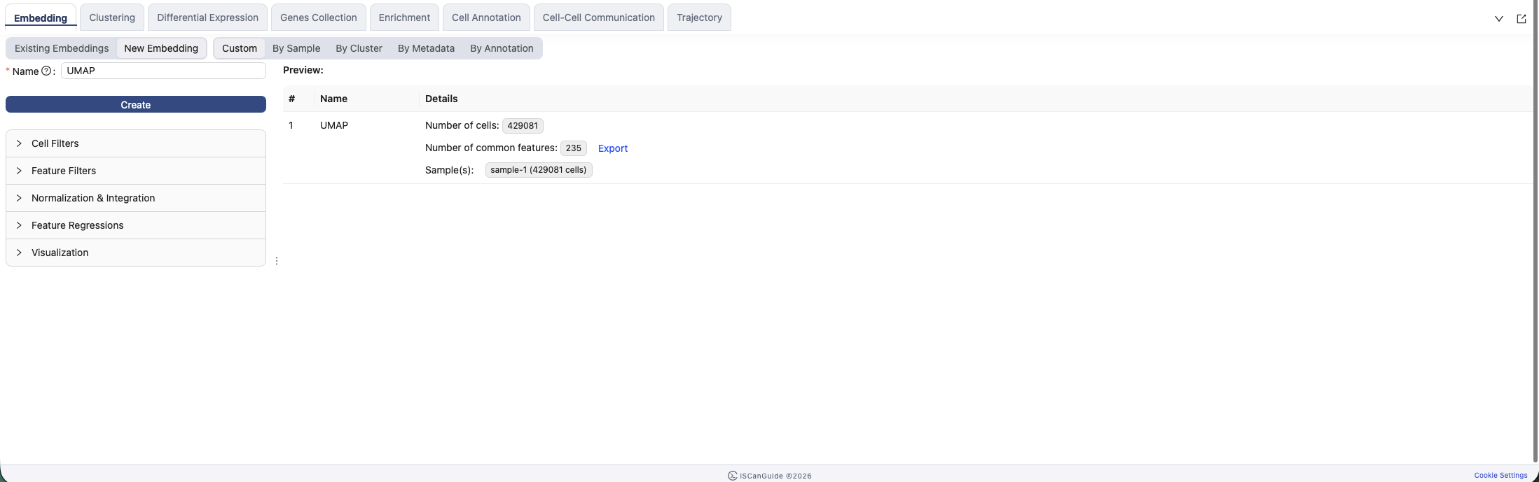
The preview lists every embedding that will be created, with its resolved name and its cell and feature counts. This is where you see what your placeholders became. If your filters leave an embedding too small to build, it is flagged here instead of failing later. Click Create when the list looks right.
11Existing embeddings
Completed embeddings are listed with the samples and cell counts they cover. Expand one to see every parameter it was built with, and rename it if you want.
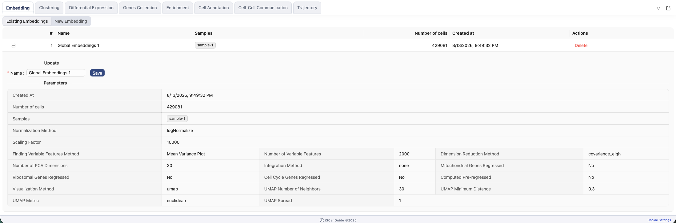
Note: if Compute Pre-Regressed Data for Comparison was enabled, View shows the before and after comparison.